Residual Plots
The function will analyze the residuals of a linear regression.
Choose Stats > Residual Plots

X Y Values: Select two different columns for the predictor (X) and the response variable (Y). Only residual plots will be displayed; the linear regression of the two variables is performed in the background and will not be shown.
In linear regression, residuals are the differences between the actual observed y-values and the predicted values from the fitted line. They represent how far each data point deviates from the line—some points fall above the line (positive residuals) and others fall below (negative residuals).
The assumption that residuals should be normally distributed is crucial because it informs us about the nature of the “noise” or random variation in the data. When fitting a line to data, the line is considered to represent the true relationship, plus some random error. If these errors (residuals) follow a normal distribution, it suggests that the scatter around the line is due to natural random variation, rather than a systematic pattern that might have been overlooked. This normal distribution of residuals is expected if many small, independent factors are affecting the measurements.
When residuals aren’t normally distributed, it often indicates a problem with the linear model. It might suggest a missing important curved relationship, omitted key variables, or the presence of outliers that are influencing the line in unexpected ways. This is why checking residual normality is a standard diagnostic tool—it helps validate whether the linear regression assumptions are reasonable. Both Minitab and JMP provide tests and plots to check this assumption, assisting users in determining if their linear model is appropriate for their data.
Normality of Residuals
Shapiro-Wilk Statistics 0.968   p-value 0.015
Anderson Darling Stats. 1.174   p-value 0.004
p values are the probabilities of true dist is normal.
The p-value in the results indicates the probability of the residuals coming from a normal distribution. When the p-value is higher than the significance level, the residuals are likely to have a normal distribution. Conversely, when the p-value is smaller than the significance level, the null hypothesis should be rejected, suggesting that there may be more than random errors in the residuals.
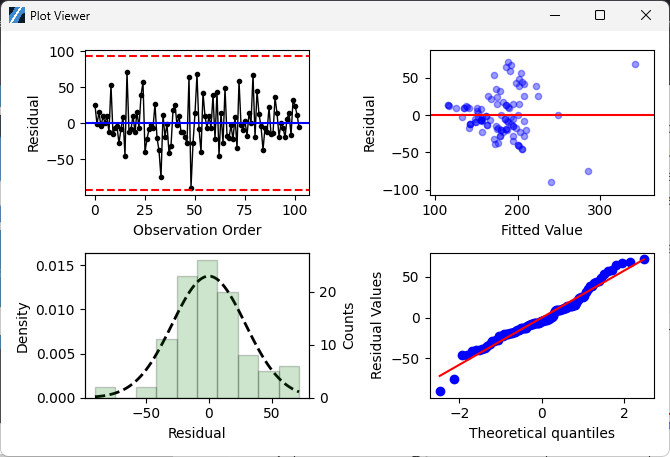
Residuals versus order: This plot displays the residuals in the order the data were collected.
Use this plot to verify the assumption that residuals are independent. Independent residuals show no trends or patterns over time. Ideally, residuals should fall randomly and not exceed the red dashed lines.
Patterns may indicate that residuals near each other are correlated and not independent.
|

|
|
If you see a pattern, investigate the cause. The above types of patterns may indicate that the residuals are dependent.
Residuals versus fits: This graph plots residuals on the y-axis and fitted values on the x-axis. Use it to verify that residuals are randomly distributed with constant variance.
Ideally, the points should fall randomly on both sides of 0, with no recognizable patterns in the points.
The patterns in the following table may indicate that the model does not meet the model assumptions.
Fanning or uneven spreading of residuals across fitted valuee means Nonconstant variance
Curvilinear menas A missing higher-order term
A point that is far away from zero means An outlier
A point that is far away from the other points in the x-direction means An influential point
Histogram of residuals: This shows the distribution of residuals for all observations. Use it to determine if data are skewed or include outliers.
A long tail in one direction indicates Skewness
A bar that is far away from the other bars indicates An outlier
A histogram is most effective when you have approximately 20 or more data points. If the sample is too small, then each bar on the histogram does not contain enough data points to reliably show skewness or outliers.
Normality QQ Plot: This plot displays residuals versus their expected values if normally distributed. Use it to verify that residuals are normally distributed. The plot should approximately follow a straight line.
Check out the help page of Normality for more information about QQ plot interpreting. LINK
If a nonnormal pattern is observed, use other residual plots to check for issues like missing terms or time order effects. Non-normal residuals can lead to inaccurate confidence intervals and p-values.